4  Individual Documents

The easiest way to get started with Quarto is to create stand-alone documents. These are self-contained documents, incorporating formatted text and executable code in a single file.

To create a new document with Quarto, you can simply use the menu options in RStudio or MS Visual Code, or create a file with the extension .qmd.

4.1 Creating a document with RStudio

Before you start, make sure you have installed the Quarto software on your machine. It is a standalone software program, which needs to be installed for the rest of the process to work (see the Section 1.4 section).

If you already have a recent version of RStudio installed, you will need to install the following packages for the example:

install.packages("tidyverse")
install.packages("palmerpenguins")
install.packages("quarto")

Now, in RStudio we create a new project choosing the Quarto project option, as it appears in Figure 4.1.

Figure 4.1: New Quarto project

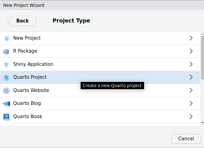
We can name our project directory as first-example and click Create Project.

As a result, a new project should appear open on the screen, with the appearance shown in Figure 4.2.

Figure 4.2: First example

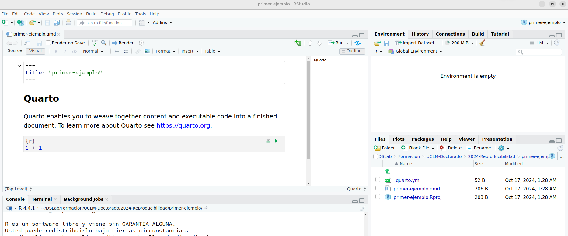
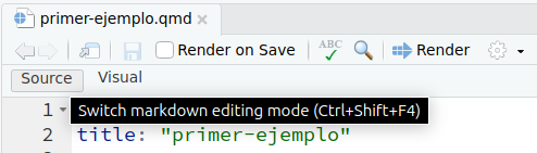
Specifically, in the upper left panel we can see that, by default, the Visual editor has been opened, which allows creating Quarto documents in a more intuitive way. However, to start getting familiar with the structure of a quarto document from the beginning, we will switch to the Source editor to view the source code, by clicking on the button shown in the figure Figure 4.3.

Figure 4.3: Source editor

4.2 Document structure

The following example code presents a basic structure of an individual Quarto document.

---
title: "My first document"
author: John Doe
date: 2024-12-20
---

Here we have a line of formatted Markdown content.

```{r}
#| label: my-label

# This is a code chunk. You can place here executable
# code that will be run by the R interprenter. By default, the final
# document will automatically integrate both the input code and the
# output from its execution
a <- 1 + 1
```

*Additional* Markdown content after the code chunk.

The file content consists of two parts:

• Preamble: is delimited by two --- tags. Within this area we can assign values ​​to configuration options for layout and creating the document, such as title, author(s), date, etc.

We can also configure various options related to the output format of the documents.

• Document body: is composed of text paragraphs formatted using the Markdown markup syntax, which we will see later. In addition, executable code fragments or chunks can also be inserted into the text, which are marked up using a special syntax (as we see in the example above).

Each chunk of executable code is delimited as follows:

```{r}
# Código en R
```

Support for additional programming languages

Although in this workshop we focus on the R language, you should know that Quarto also supports other programming languages ​​such as Python, Julia or Observable.

We can change the programming language of each code chunk by indicating its name at the beginning, for example:

```{python}
# Código en Python
```

Nevertheless, this code chunk in other languages requires additional configuration. For example, we must set up a Python interpreter to execute code chunks written in this language.

4.2.1 The preamble

A basic example of a preamble is as follows (although it would be sufficient to simply provide a title for the document):

---
title: "My first document"
author: John Doe
date: 2024-12-20
---

Of course, more options can be added, which we will explain next

4.2.2 List of options

There is an extensive list of configuration options that we can include in our documents.

• HTML output options: these allow us to configure various basic aspects of the document, such as the title and subtitle, date, author (or list of authors), summary or DOI; formatting options such as the subject or advanced styles for HTML content with CSS; numbering and table of contents, etc.

• Basic options for HTML with Quarto.

• Complete list of HTML options with Quarto.

• PDF output options: these offer the possibility of configuring multiple parameters for the creation of the document in this format, many of them similar to those for the HTML output. A particularly relevant option is to choose the LaTeX document format (documentclass option), which defines the general appearance of the layout to be used. By default, classes from the KOMA Script metapackage are used, such as scrartcl or scrbook. It is also important to indicate the papersize option, in our case to ensure that a standard format is used such as A4. The citation format is also relevant, being able to choose, for example, the BibLaTeX engine which is more powerful, with multilingual support and for native UTF-8 character encoding. Finally, it is also important to indicate the compilation engine. If you want full flexibility in document layout, it is highly recommended to use the XeLaTeX engine (option pdf-engine: xelatex), which is the default used by Quarto.

• Quarto PDF Basics.

• Complete list of PDF options available with Quarto.

4.2.3 Basic Markdown syntax

In the following link you can find a quick basic tutorial that shows the basic options of the Markdown syntax accepted in Quarto documents to format textual content.

• Basic guide to markdown syntax.

4.3 Creating documents (output)

By default, if we do not indicate anything, Quarto will generate a single output format of the document in HTML. However, it is possible to define more than one output format by including more configuration options. Of course, you can indicate different options to generate several output formats simultaneously, or to choose the output format that we want to produce based on our interests, selecting the format that we need when previewing or when generating the final document.

4.3.1 Preview

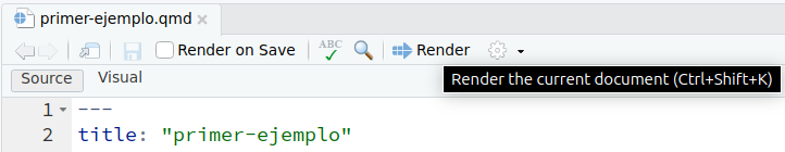
To preview the document we have to press the Render button in the tools menu of the RStudio interface, as shown in Figure 4.4.

Figure 4.4: Render button to preview the generated document.

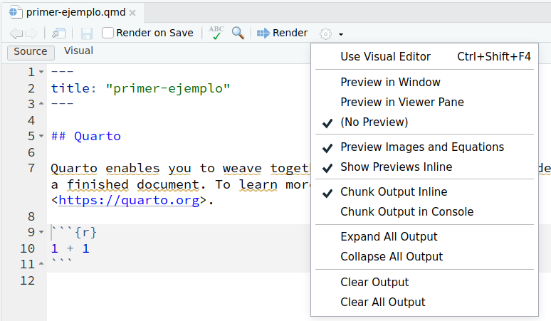
By default, our main web browser or a panel in the RStudio interface will open showing the HTML page with the document already generated. By clicking on the gear icon next to the Render button we can select, among other things, the type of preview we want to be launched after completing the creation of the document or completely disable said preview. Available options are shown in Figure 4.5

Figure 4.5: Render operation preview options.

4.3.2 Selecting output type

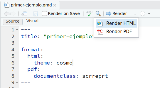
When we have several output format options configured in our document, we can choose at preview time which of the formats is chosen to generate the document. In the Figure 4.6 you can see an example of a document that includes settings for two output formats (HTML and PDF) and the change in the Render button, in which a small black arrow now appears just to the right of the button icon to display the two available output options.

Figure 4.6: Selecting output formats with the Render operation.

4.3.3 Basic configuration options

Below is an example of some basic configuration options that are typically found in documents formatted as HTML output.

---
title: "My first document"
author: 
  - "John Doe"
  - "Mary Jane"
date: 2024-12-20

lang: en
bibliography: references.bib

format:
  html:
    theme: cosmo
    toc: true
    number-sections: true
    html-math-method: katex
    css: styles.css
  pdf:
    documentclass: scrreprt
---

REST OF THE DOCUMENT

In this example, in addition to the author and the date, a list of two authors is indicated, the main language of the document (Spanish), the bibliography reference file (in .bib format) and, within the HTML options, the layout topic, the inclusion of a table of contents (located by default at the top right), section numbering, selection of the engine to render equations in the document and a custom styles file in CSS format to adjust some fine layout options.

One option worth highlighting is to force all resources (images, style information, etc.) to be integrated into the HTML file itself, to facilitate direct sharing or publication of the document without having to also provide the auxiliary files necessary to display it in the browser. This option is shown below:

format:
  html:
    embed-resources: true

4.4 Executable code chunks

The most distinctive feature of documents created with Quarto is the possibility of inserting executable code fragments, called chunks, into the document itself. This also includes the option for said code to generate different results (numeric, graphic, tables, animations, etc.) that are integrated directly into the document. In this way, if we keep the code updated, the correct versions of said results will always be generated.

The executable code fragments have the following structure:

```{r}
#| label: id-fragmento

# Aquí va el código ejecutable
a = c(1, 2, 3, 4)
b = a^2
```

The triplet of characters ``` is called a fence and delimits the beginning and end of the code fragment. Immediately after the opening delimiter, the identifier of the programming language in which the code of that fragment is written is written in curly braces. This information is used to choose the appropriate syntax highlighting to display the code of that language and to select the interpreter that executes the code and produces the results.

In the following lines we can include one or several configuration options specific to that code fragment, using the syntax #| option: value. For example, in the previous fragment the option #| label: fragment-id creates a label (which must be unique) to identify that fragment of code within the document.

• List of options for code fragments.

Some frequently used options are:

• eval: true | false | [...]: Indicates whether the content of that snippet should be evaluated (executed). A list of positive or negative line numbers can be passed to explicitly select which lines of code are included (positive) or excluded (negative) from execution.

• echo: true | false | fenced | [...]: Indicates whether the source code of the snippet should be included in the document or not. The fenced option also includes the cell delimiter as part of the output. Finally, it also accepts a list of positive or negative line numbers to select which lines of code will or will not be displayed in the snippet.

• output: true | false | asis: To decide whether the result of the code execution is included in the document or not. The asis value forces the result to be treated as raw Markdown content.

• warning: true | false: Indicates whether warning messages should be included in the output.

• error: true | false: Indicates whether generated error messages are included in the output.

• message: true | false: Indicates whether generated information messages are included in the output.

When fragments generate figures, these are inserted into the document itself. Let’s look at an example:

```{r}
#| label: fig-example-cars
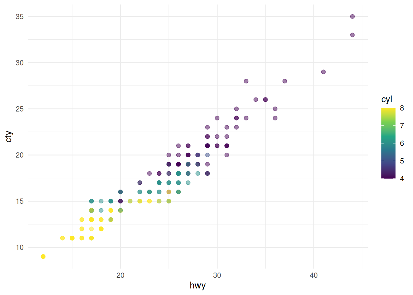
#| fig-cap: "Gráfico de correlación lineal positiva entre el kilometraje en ciudad y en carretera de diferentes modelos de coches."

library(ggplot2)
#| label: scatterplot
#| echo: true

ggplot(mpg, aes(x = hwy, y = cty, color = cyl)) +
  geom_point(alpha = 0.5, size = 2) +
  scale_color_viridis_c() +
  theme_minimal()
```

Figure 4.7: Gráfico de correlación lineal positiva entre el kilometraje en ciudad y en carretera de diferentes modelos de coches.

Automated figure numbering

It is important that the fragment identifier we choose for the code that generates one or more figures begins with the prefix fig-.

In this way, we ensure that Quarto automatically assigns a number to the generated figure and that we can create cross-references (internal links) to that figure in our document.

As we will see later, other output types such as tables also need to be assigned a specific pattern in their fragment identifier so that they are automatically numbered and can be referenced within the document.

Figure management in Quarto is quite sophisticated, to the point that you can easily organize several subfigures with their respective individual descriptions, as shown in the following example using some additional options.

```{r}
#| label: fig-mpg-subplot
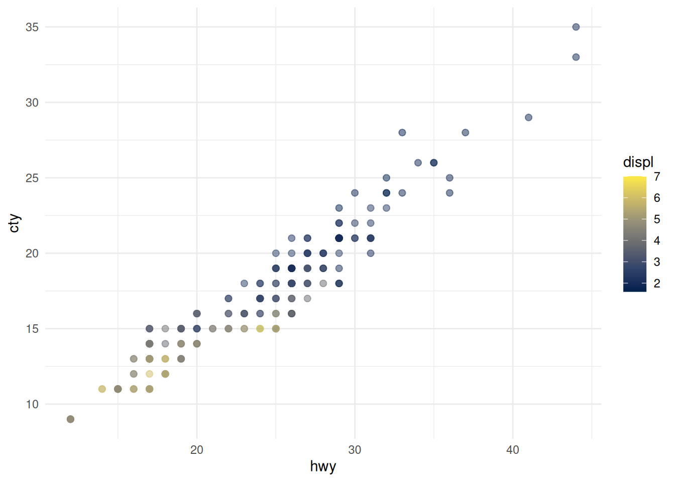
#| fig-cap: "City and road mileage of 38 popular car models."
#|
#| fig-subcap:
#|   - "Color by num. of cylinders."
#|   - "Color by motor displacement."
#| layout-ncol: 1

ggplot(mpg, aes(x = hwy, y = cty, color = cyl)) +
  geom_point(alpha = 0.5, size = 2) +
  scale_color_viridis_c() +
  theme_minimal()

ggplot(mpg, aes(x = hwy, y = cty, color = displ)) +
  geom_point(alpha = 0.5, size = 2) +
  scale_color_viridis_c(option = "E") +
  theme_minimal()
```

(a) Color by num. of cylinders.

(b) Color by motor displacement.

Figure 4.8: City and road mileage of 38 popular car models.

Some common options for chunks that generate figures are:

• fig-width: Width of the figure.
• fig-height: Height of the figure.
• fig-cap: String in quotes to be inserted as a caption.
• fig-alt: Alternative text message that fills the alt attribute of the HTML image (for example, to improve the accessibility of the content).
• fig-dpi: Resolution setting of the figure (in dots per inch).

The tutorial on executable code snippets in the official documentation presents more information and examples on how to use this powerful Quarto feature.

4.5 Author toolkit

In addition to the ability to integrate executable code and its results into our scientific papers, Quarto includes a number of resources and tools to provide a complete and efficient authoring experience.

4.5.1 Document sections

As we saw in the Section 4.3.3 example, there are two HTML document configuration options that allow us to number sections and incorporate an automatically generated table of contents at the top right of our document.

format:
  html:
    toc: true
    number-sections: true

An important feature for creating scientific documentation is being able to include cross-references, that is, links that take us to other sections of the document. In Quarto this is achieved by following a simple procedure in two steps:

1. We add a unique tag to identify the section with the syntax:

## Section header {#sec-tag}

2. We reference the tag we created for that section in another part of the text, so that Quarto automatically creates the link (cross-reference) to that section:

In the text we add a reference to the @sec-tag.

An example of this type of automatically created cross-reference can be seen at the beginning of this section. On the other hand, if we want a section of the document to be excluded from the numbering scheme of the rest of the sections, we use the special tag in the title of that section:

## Unnumbered section {.unnumbered}

There are several additional options that control the way and style in which sections are created and numbered. Some of them are:

• anchor-sections: Causes an anchor link to be displayed (to link directly to that section in another document) when the mouse hovers over a section title.
• toc-depth: Specifies how many levels deep the section numbering appears in the table of contents. By default, 3 levels are displayed.
• toc-location: body | left | right | left-body | right-body: Controls the location where the table of contents appears in the document.
• toc-title: String with the title of the table of contents.
• toc-expand: Indicates whether all sections in the table of contents should be expanded or collapsed so the user can click on the ones they want to expand.
• number-depth: Determines the maximum depth to which sections in the document are numbered (note, this should be in line with the value assigned to the toc-depth option).
• number-offset: Allows you to set the number at which sections are numbered. If we want the document to start numbering the highest level section as “4” then we use number-offset: 3. If we want the document to start at a level 2 section numbered “1.5” we must specify number-offset: [1,4]. Setting a value for this option means that number-sections: true is automatically set.

4.5.2 Equations

Another essential aspect of scientific documents is the appearance of mathematical symbols, formulas, and equations. There are several HTML libraries that allow properly formatted equations to be displayed on the screen. For its part, LaTeX, due to its origins, has always included powerful and versatile tools to handle this type of content, so support is guaranteed for PDF documents.

In general, the syntax used to write equations is very similar to that used in LaTeX.

• Tutorial on mathematical expressions in LaTeX.
• Summary of mathematical syntax in LaTeX.

There are two ways to display equations in our content, also following a similar philosophy to that of LaTeX documents:

• Equations in line with the text: to display the equation within a line or paragraph, at the same height as the rest of the text.
• Equations in display mode: the equation is displayed in a separate space, between two paragraphs of text and with a certain margin of space at the top and bottom.

Example of an inline equation: $F = m \cdot a$

Result: example of an inline equation: \(F = m \cdot a\).

Example of an equation in display mode:

$$E = mc^{2}$$

Which produces the following result (see below how to add the numbering):

\[ E = mc^{2} \tag{4.1}\]

If we also want to number our equations, we must remember to use the unique identifier tag pattern eq-tag to identify it and then be able to insert internal references to said equation in the text.

$$ E = mc^{2} $$ {#eq-energy}

As a result, we can insert a cross-link to Equation 4.1.

4.5.3 Tables

Tables are another relevant content that we can format in different ways in the documents generated with Quarto.

• Introduction to creating tables in Quarto.

In this case, the visual editor can greatly simplify this task for us. It is advisable to try it to see the difference, since it is a very intuitive tool. However, following the same line as the rest of the workshop, here we will describe the details to create this content directly in the Markdown code of the file.

The most direct way to create a table in Markdown is to compose a pipe table, so called because its syntax is based on the | operator on the command line. Let’s see an example.

| Default | Left | Right | Center |
|---------|:-----|------:|:------:|
| 1       | 2    |     3 |    4   |
| 22      | 23   |    24 |   25   |
| 4       | 3    |     2 |   1    |

The result of including the previous code in our document is:

Default	Left	Right	Center
1	2	3	4
22	23	24	25
4	3	2	1

We can see how the key to controlling the horizontal alignment of the table content is to properly place the : symbol on the line just below the title line, which separates it from the body of the table. If we do not want to include a title, it is mandatory to include the first line, but we can leave the cells blank.

Below the table we can insert the expression : Table Caption to include a descriptive message. It is also possible to directly use some style elements included in the classes of Bootstrap, the web style framework that Quarto uses to compose pages (we have seen before how to use the document option theme: cosmo to use the Cosmo theme of Bootstrap). There are different effects, and one of the most frequent is to color the background of the rows in gray alternately as well as highlight the row on which the mouse arrow is placed. These two effects are .striped and .hover, respectively.

| Default | Left | Right | Center |
|---------|:-----|------:|:------:|
| 1       | 2    |     3 |    4   |
| 22      | 23   |    24 |   25   |
| 4       | 3    |     2 |   1    |

: This is the table caption. {.striped .hover}

This is the table caption.

Default	Left	Right	Center
1	2	3	4
22	23	24	25
4	3	2	1

Finally, similar to what we do to internally reference equations and figures in our document, we can also label tables using the pattern #tbl-label to reference it as @tbl-label which is formatted like this: Table 4.1.

| Default | Left | Right | Center |
|---------|:-----|------:|:------:|
| 1       | 2    |     3 |    4   |
| 22      | 23   |    24 |   25   |
| 4       | 3    |     2 |   1    |

: This is the table caption. {#tbl-label .striped .hover}

Table 4.1: This is the table caption.

Default	Left	Right	Center
1	2	3	4
22	23	24	25
4	3	2	1

The same tag pattern should be used in the code chunk identification option #| label: tbl-label if we later want to reference the table generated by that code chunk with a cross-reference.

More details can be found on creating subtables, changing caption location, as well as creating grid tables that use a different syntax and allow arbitrary block elements to be included in each cell (multiple paragraphs, code blocks, unnumbered or numbered lists, etc.).

+-----------+-----------+--------------------+
| Fruit     | Price     | Benefits           |
+===========+===========+====================+
| Bananas   | $1.34     | - wrapping         |
|           |           | - brilliant colour |
+-----------+-----------+--------------------+
| Oranges   | $2.10     | - rich in vitam. C |
|           |           | - tasty            |
+-----------+-----------+--------------------+

: Sample grid table.

Sample grid table.

Fruit	Price	Benefits
Bananas	$1.34	wrapping brilliant colour
Oranges	$2.10	rich in Vitam. C tasty

4.5.4 Callouts

It is possible to include callout blocks, to highlight practical notes, warnings, or tips of special interest. In addition, a title is often given to the callout to make it even more informative.

::: {.callout-note}
## Callout title

There are five different types of callouts:
`note`, `tip`, `warning`, `caution`, and `important`.
:::

Callout title

There are five different types of callouts: note, tip, warning, caution, and important.

• Introduction to using callouts in Quarto.

4.5.5 Bibliographic references

The management of bibliographic references in Quarto is done by encoding the information in BibTeX format. This allows you to use any of the bibliographic citation formats supported by this package, or to include a CLS file that defines a standard format (APA, Chicago, IEEE, etc.).

For example, the document options

---
title: "My Document"
bibliography: references.bib
csl: nature.csl
---

indicate a references.bib file where we can store the information about bibliographic references (which we can obtain from Google Scholar, Zotero or other tools and services on the Internet), as well as a citation style file nature.cls (style defined by the Nature publisher).

• CLS repository with citation styles.
• Zotero repository with citation styles.

Depending on the style and format of the citation, we can use one or another syntax to indicate the author and the year in parentheses, the author outside the parentheses, page numbers, chapters, etc.

• Quarto citation syntax reference table.

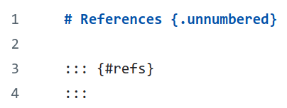
Finally, the ordered list of bibliographic references (according to the citation style criteria we have selected) must appear at the end of the document. To achieve this in an HTML document, we must include a special code, which is normally placed in a separate, unnumbered section, as shown in Figure 4.9.

Figure 4.9: Syntax to display bibliographical references at the end of the document.

When the generated output is in PDF format and the BibLaTeX or natbib reference management engines are used, then the list of references always appears at the end of the document and the previous tag is ignored. Finally, in the rare case that we do not want to include any bibliographical references in our document, we can include in the header metadata the option suppress-bibliography: true.

4.5.6 General document style

So far, the example document we have shown as well as these notes always use a style format or theme from the Bootstrap web development environment, called cosmo. However, there is a wide list of alternative themes to modify the general style of our document (color scheme, typography and font size, organization of content, appearance of links, etc.). The Quarto project is responsible for regularly combining the most popular style themes so that they are available as an option for the document.

In this theme directory on GitHub you can check an updated list of the possible values ​​that we can assign to the theme option in the header of the document. It is useful to experiment with various options to find the one that best suits the type of document generated, its content and the audience it is intended for.

An online demo of many of the available themes can be accessed on the website https://bootswatch.com/.